
台风引起南海北部海洋环流和温度变化研究取得进展
发布时间:2022-11-10 发布人:U团队
近日,海洋生态环境对台风的响应研究取得进展,相关成果Study of storm-induced changes in circulation and temperature over the northern South China Sea during Typhoon Linfa发表于海洋学领域SCI期刊Continental Shelf Research上。论文第一作者和通讯作者分别为加拿大达尔豪斯大学Yi Sui 隋艺和Jinyu Sheng 申锦瑜教授,广州海洋实验室教授、广东省海洋生态环境遥感中心主任Danling Tang 唐丹玲博士和清华大学国际研究生院Jiuxing Xing 邢久星教授共同完成该研究。

本研究利用观测数据和海洋数值模型(ROMS-nSCS)方法研究了2009年南海北部台风“莲花”的水动力响应过程。基于区域海洋大陆架环流数值模型(ROMS-nSCS)用于定量 分析台风“莲花”过境前后上层海洋环流和温盐场变化的重要物理过程。ROMS-nSCS的大气强迫场数据来自气候再分析系统(CFSR),同时,在CFSR的大气强迫中插入了一个参数化的涡旋,以提高台风“莲花”过境时风场与海平面气压数值 的准确度。ROMS-nSCS的横向开放边界条件是根据混合坐标海洋模式(HYCOM)产生的全球海洋环流再分析指定的。ROMS-nSCS模式产生的结果显示,上层海洋环流的特点是在直接受“莲花”影响的区域上有强的风生流,在“莲花”横扫过的地区中存在强烈的近惯性振荡(NIOs)。模拟的台风后的降温 主要发生在台风路径的右侧,这与卫星分析数据相吻合。此外,模拟的NOIs也有明显的右偏。模式流场的旋转谱分析结果表明背景场环流的涡度可引起NIOs的峰值频率fp比局地惯性频率高约9%左右。对模式结果的分析还显示,台风“莲花”导致的海温降低来自多个海洋动力阶段响应。在“莲花”的早期发展阶段,台风过后的降温主要受台风引起的垂直方向上的平流的影响。在“莲花”成熟期,台风导致的降温主要来自于台风引起的混合及平流的联合效应。台风引起的升温发生在台风“莲花”影响区之外区域,主要由台风诱发的下降流引起。
该研究由广东省特支计划U团队项目(2019BT02H594)、国家自然科学基金面上项目(41876136)等资助。
该研究成果进一步丰富、深化了风泵的生态环境效应理论。
论文链接:https://doi.org/10.1016/j.csr.2022.104866
论文PDF 见NO.179:http://www.lingzis.com/journal article.htm

Fig. 5. Distributions of daily mean sea surface temperatures (SSTs) and surface currents produced by (left panels) the ROM-nSCS and (middle panels) HYCOM reanalysis and (right panels) SSTs calculated from the daily satellite remote sensing data on (top) 16, (central) 19, and (bottom) 22 June 2009. For clarity, surface current vector in right (middle) panels are plotted at every 9th (6th) model grid point of the ROMS-nSCS (HYCOM). The black box in c3 shows the region of AADL.

Fig. 13. Distributions of (a1,b1,c1) ΔU→A+M and ΔTA+M, (a2,b2,c2) ΔU→M and ΔTM, and (a3,b3,c3) ΔU→A and ΔTA at the sea surface at 00:00 on (a1-3) 19, (b1-3) 20 and (c1-3) 21 June 2009, respectively. The red dashed line in each panel represents the storm track. For clarity, surface current vectors are plotted at every 9th model grid point.
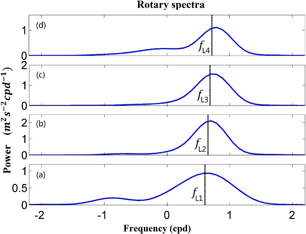
Fig. 16. Rotary spectra of simulated surface currents at locations (a) L1, (b) L2, (c) L3, and (d) L4. The vertical dashed line in each panel represents the local inertial frequency at the location. The negative frequency represents the counterclockwise components.

Fig. 17. Evolving rotary spectra of simulated surface currents at locations (a) L1, (b) L2, (c) L3, and (d) L4. In each panel, the green line represents the effective frequency (fe = f + ζ /2), the yellow dashed line represents the local inertial frequency (f), and the blue line represents the peak frequency (fp) at each location. ERS are calculated using a 10-day sliding window. The frequency axis is limited to the near-inertial band.